AI-based weather forecasting is an emerging paradigm different than numerical weather prediction (NWP), which today is the default way of making weather forecasts. In some cases, their performance is on par or exceeding that of NWP, especially in the longer term. However, AI-based weather forecasts tend to be smoother than NWP forecasts. What’s more, they seem to become even blurrier at longer lead times. This impacts weather forecasts: for example, extreme weather events are captured less precisely. In this article, we’re going to explore why this occurs. Then, we continue with reviewing solutions, allowing the quality of AI-based weather forecasts to improve.
How AI-based weather models are trained
Before we look at the sharpness of AI-based weather forecasts, it’s good to briefly revisit how they are made in the first place.
As a simple example, suppose that we are trying to model how the atmosphere evolves between now and an hour from now – from time T to time T+1, as visualized in the image below. AI-based weather models take a representation of the atmosphere at time T – by combining various elements at various vertical levels – as model input. Typically, this is an analysis generated by an NWP model. This leads to a prediction, in other words the expected state at time T+1. When training is in the early stages, this prediction is often quite wrong. It is compared with the true state at T+1, the ground truth. This leads to a loss value, which tells us how poorly the model performs at that moment. Using mathematical techniques, given the loss and the input, the so-called weights of the AI-based weather model are slightly altered. We then start again with the input, doing the same repeatedly, until a working model emerges. It is not uncommon that this takes a few weeks using many powerful computers, with hundreds of thousands of such iterations, while success is not guaranteed.
Training AI-based weather models does not involve using just one example. Typically, many years of atmospheric analysis data are used, as there is a large variation in possible weather conditions that models need to account for. It is not uncommon to see that models are trained with 40 years of data, typically using the ECMWF Reanalysis v5 (ERA5) dataset.
When trained, generating a new worldwide weather forecast for the variables the model was trained with is fast. Using a new analysis at some time T, the model is used to make the prediction for the next timestep T+1. That prediction is then used autoregressively to make the prediction for timestep T+2, and so forth. These days, time steps of 6 hours are common – in other words, moving from T to T+6, then to T+12, and so forth. Making a two-week weather forecast, using the right hardware, takes just a few minutes.
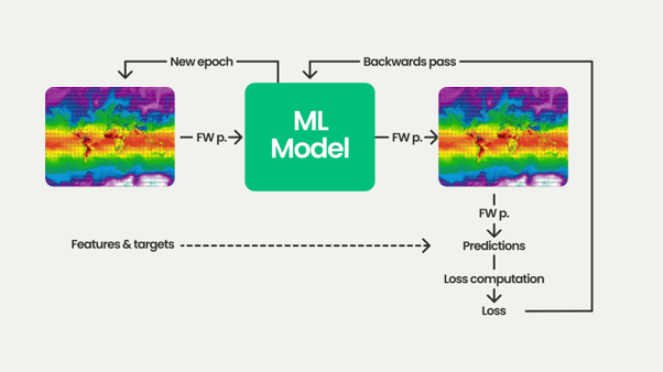 Figure 1: training an AI-based weather model
Smoothing and error accumulation in AI-based weather forecasts
Before, we have already read that forecasts are typically less detailed (as compared to NWP forecasts) to begin with, and that they can lose their sharpness even more with forecasts for longer lead times. Let’s now look at these two problems individually.
Training for average performance: smoothing effects
Recall from the previous section that the differences between the prediction and the true state (the expected prediction) of all the training samples are represented in a loss value. Since this value must be computed, there must be a function doing so: we call that function the loss function. Choosing a loss function is at the discretion of the model developers and helps optimize models in a desired way.
In AI-based weather models, many times, a customized Mean Squared Error loss function (or something that looks like it, such as Root Mean Squared Error) is used. In the simplest form, MSE loss looks like the formula below (Versloot, 2019). For all grid cells, the prediction is subtracted from the expected value from the training data, the difference is squared, and the sum over all grid cells is then divided by the number of grid cells to compute the average. In other words, MSE losses compute the average error across the whole prediction (in the case of AI-based weather models, that is the global weather prediction for a time step).

Figure 2: MSE loss.
Recognizing meteorological effects and the expressiveness of NWP models (providing the analysis data for training) around the poles, AI weather model developers typically customize their loss functions even further, taking these effects into account. For example, the loss function below – that of the GraphCast weather model – considers forecast date time, lead time, spatial location and all variables when computing loss. Nevertheless, as can be seen from the right of the function, it is still a squared error – and thus an MSE loss.

Figure 3: GraphCast loss function (Lam et al., 2022).
Now, recall from the previous section that the loss value, through the optimization process after each step, guides the direction of model optimization. In other words, if a loss function is used that penalizes errors (and especially large errors, given the square), it is no surprise to see that smoothed, average forecasts tend to produce lower error values than detailed forecasts capturing both signal and noise. After all, on average, average forecasts produce the lowest errors – as detailed forecasts can be very spot-on but produce large MSE scores if they are wrong instead. The figures below visualize this effect. For some expected temperature forecast, if a fictional model produces a more average, smoothened prediction, the resulting MSE is (much) lower compared to a detailed one. Even though it also captures the larger-scale signal, it produces a lot of small-scale errors when doing so, which are penalized heavily by the square present in MSE loss functions.

Figure 4: a smoothened temperature forecast has an MSE of 338.06.

Figure 5: a more detailed forecast capturing the signal while being noisy has a much larger MSE.
In many cases, this is not a problem: average weather tends to be represented well in the many years of training data and weather conditions tend to be like averages. More problematic is the case of extreme weather.
First, extreme weather does not happen often (hence the name), so it is underrepresented in the training data, making its prediction difficult. What’s more, since models are trained to reduce the average error, and average predictions tend to produce lower average errors (see the figures above), what follows is that models tend to produce forecasts where extreme events are underestimated. A case study of the Pangu-Weather model in extreme weather events demonstrates this effect (Bi et al., 2022). In other words, one of the downsides of AI-based weather models is that they can be quite good ¬and sometimes even better – in average scenarios, such as large-scale weather systems and their positions. NWP models still provide more detailed forecasts for small-scale phenomena, such as extreme weather events and local differences in wind speed, as can e.g. be seen in figure 6.

Figure 6: the energy spectra plot for 10-meter windspeed at short lead times (+12 hours in this case) indicates that IFS HRES has more power, thus more detail, for small-scale weather phenomena compared to AI-based models: this includes expressivity for small-scale extreme weather conditions.
Error accumulation: less detailed forecasts with time
In our article about evaluating AI-based weather models with WeatherBench we already briefly encountered energy spectra, which can be used to estimate the amount of detail present in a forecast. Recall that weather is both large-scale and small-scale at the same time: a larger-scale weather system (such as a low-pressure area) can bring different types of weather to different regions (for example, snow in some part of the country; rain in another).
If a weather model is good in expressing these small-scale weather phenomena, its power in the energy spectrum in the shorter wave lengths is higher. One of the shortcomings of AI-based weather models is that they tend to produce blurrier forecasts with longer lead times. This can be seen in the energy spectrum below, which visualizes the power spectrum for various NWP-based and AI-based weather models for 8 days in the future for 2-meter temperature. IFS HRES, the ECMWF NWP model, has the highest power at small wave lengths, with a significant difference when compared to the AI-based weather models and the ensemble mean. In other words, small-scale weather phenomena are currently expressed better in NWP models than in AI-based weather models.

Figure 7: Power spectra for various deterministic AI and NWP weather models for 2-meter temperature at 192 hours ahead (8 days). Higher power means that forecasts have more detail. Shorter wavelength means lower scale, thus higher power at shorter wavelengths means that small-scale weather phenomena are captured with higher detail. Image from WeatherBench (2024).
The effect can also be seen when actually looking at the output of AI-based weather models. For example, in the figure below, we are comparing the forecasted temperature at 2 meters for +0h and +360h in the future using a run of the AIFS weather model. Clearly, the model is less expressive 360 hours ahead compared to 0h in the future. This is especially apparent in the Atlantic Ocean, where temperature zones seem to be more ‘generic’. This reduction in sharpness present with AI-based weather models results in lower power scores in energy spectra for lower wave lengths and, in the end, influences the quality of predictions made by these models for your location.

Figure 8: Output of the AIFS weather model as visible on our professional weather platform I’m Weather. On the left, we see the initialization of the forecast (at timestep +0h); on the right, the forecast for 15 days ahead (at timestep +360h). Observe the differences in detail when comparing smaller-scale differences in temperature between both time steps, especially in the Atlantic.
Like the smoothing effects discussed before, for improving AI-based weather modelling, it’s important to understand the origin of reduced sharpness. Effectively, it is related to the autoregressive procedure of AI-based weather modelling. That is, each weather forecast is started with an analysis of the atmosphere, which is the best possible mix between an older forecast for the starting time and observations taken since then. Using an AI weather model, this analysis is then used to generate a forecast for a future time step, e.g. for 6 hours in the future. We then use this forecast to generate the forecast for +12 hours; that one for the +18h hours forecast, and so forth. In other words, autoregressive modelling means that predictions by the AI model are used for generating new predictions.

Figure 9: autoregressive AI-based weather modelling: using a previous prediction for generating a new one.
However, recall from a previous article that all models are wrong, while some are useful. The wrong, here, originates from the observation that the prediction will always be a bit off compared to reality. The fact that predictions of AI weather models are always a bit smoothened out, as discussed in the previous section, effectively means that there is an error in the first prediction (and besides, they can be simply wrong as well). This error can also be seen as information loss, as there is a difference between reality and prediction. If you would then use this prediction for generating a new one, the information loss introduced with the first prediction due to smoothing and other causes is exacerbated in the second prediction; also in the third, and so forth. This is known as error accumulation, since additional error is introduced with every forecast step. Its visibility increases slowly: in the first few time steps, the effect is not significant, but at longer lead times forecasts get blurrier quickly. Clearly, error accumulation can be observed when comparing the analysis with the forecast for +360 hours, as we saw above!
Making AI-based weather forecasts more detailed: current approaches
While smoothing and error accumulation are a given in some of the first generation of AI-based weather models, they are not a roadblock anymore – they can be mitigated. Some of these mitigation techniques focus on reducing error accumulation, others on ensuring that extreme values are better represented in AI-based weather forecasts. Let’s take a look at a few of these developments, of which some are already built into the second generation of models.
Using training techniques to reduce error accumulation
The first, and quite straight-forward, solution is reducing the effects of error accumulation while training the weather model. This can be done in multiple ways, such as including autoregressive modelling in the training procedure, or using separate models for different time horizons.Including autoregressive modelling in training
GraphCast is one of the models which includes autoregressive modelling in its training procedure: “In order to improve our model’s ability to make accurate forecasts over more than one step, we used an autoregressive training regime, where the model’s predicted next step was fed back in as input for predicting the next step” (Lam et al., 2022). This was combined with curriculum learning, where training a model happens in multiple phases. In the first phase (1.000 iterations), the learning rate was increased slowly, allowing the model to converge in a sensible direction while increasing the speed with which it does. In the second (300.000 iterations), learning rate was reduced slowly, allowing the model to converge to the best possible loss minimum. Finally, with a very small learning rate, the model continued training for 11.000 additional iterations, slowly increasing the number of time steps predicted i.e. the autoregressive procedure. In total, the model was thus trained for 311.000 iterations; ablation results suggest that including autoregressive modelling in the training procedure indeed improves longer-term performance of the model.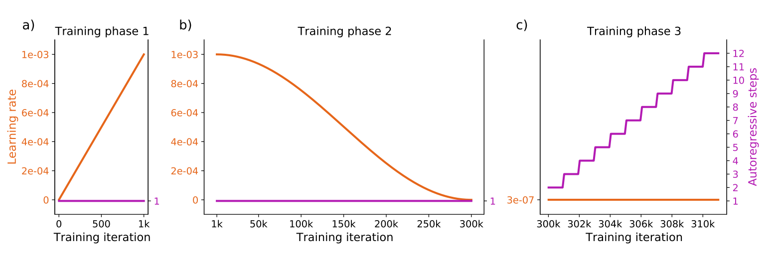
Figure 10: GraphCast training phases. Image from Lam et al. (2022).
Using separate models for different time horizons
Recall that error accumulates over time due to the long chain of autoregressive forecast steps. Chen et al. (2023b), in their FuXi model, first pretrained their model on years of analysis data for a single time step. Subsequently, the pretrained model was finetuned by including autoregressive modelling for the short term (0 to 5 days) and named FuXi Short. This model was subsequently finetuned for a longer time horizon; the resulting model is named FuXi Medium. FuXi Long is subsequently finetuned from that model and optimized for 5-to-10-day time horizons. When generating forecasts, depending on the time step, one of the three models is used. This technique, called model cascading, has demonstrably reduced error accumulation and leads to better forecasts at longer lead times.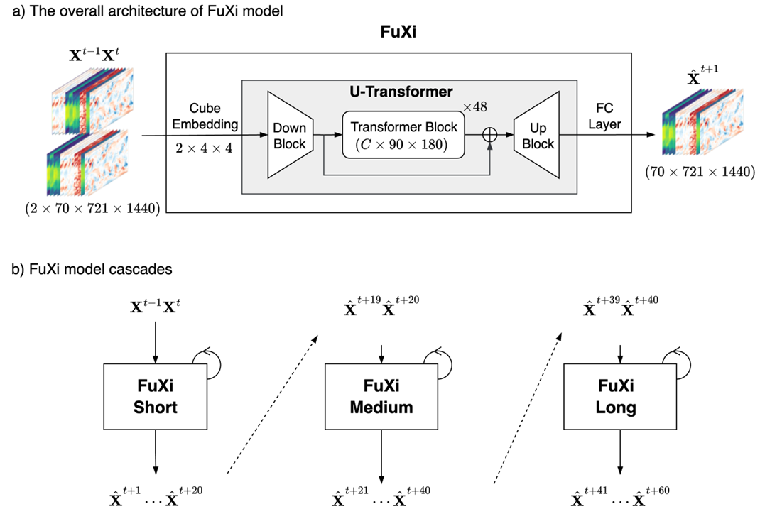
Figure 11: FuXi is a Transformer-based model, but forecast generation happens with three separate models trained on either the short term (timesteps 0 to 20), medium term (timesteps 21 to 40) or long term (timesteps 41 to 60). Image from Chen et al. (2023b).
Using ‘adapters’ to specialize for time steps
In the pretraining/finetuning paradigm followed by many of today’s AI weather models, the model weights (i.e., its parameters, its understanding about weather, its ability to make predictions) are fixed after training completes. Changing them is expensive, because that would require the model to be trained further, incurring significant computational resources to be spent. It is unsurprising to see that this problem is also encountered in other fields, e.g. when training large language models and models for computer vision.The FengWu-GHR AI weather model (a development on top of the second-generation FengWu weather model) uses a technique called Low-Rank Adaptation (LoRA) to continue finetuning without spending these resources (Han et al., 2024). In LoRA, small, adapter-like modules are added to all layers of the original model, of which the parameters are frozen. The number of added parameters (which are trainable, thus require resources) is typically only a few percent of the parameters of the original model. That way, finetuning can be done relatively cheaply.
What’s more, the finetuning approach followed for training FengWu-GHR resolves conflicting optimization differences between e.g. shorter-term and longer-term lead times, which are unaccounted for when including autoregressive modelling in training and even when using separate models for different time horizons. FengWu-GHR shows promising evaluation metrics when compared to ECMWF’s IFS model and to Pangu-Weather (Han et al, 2024).
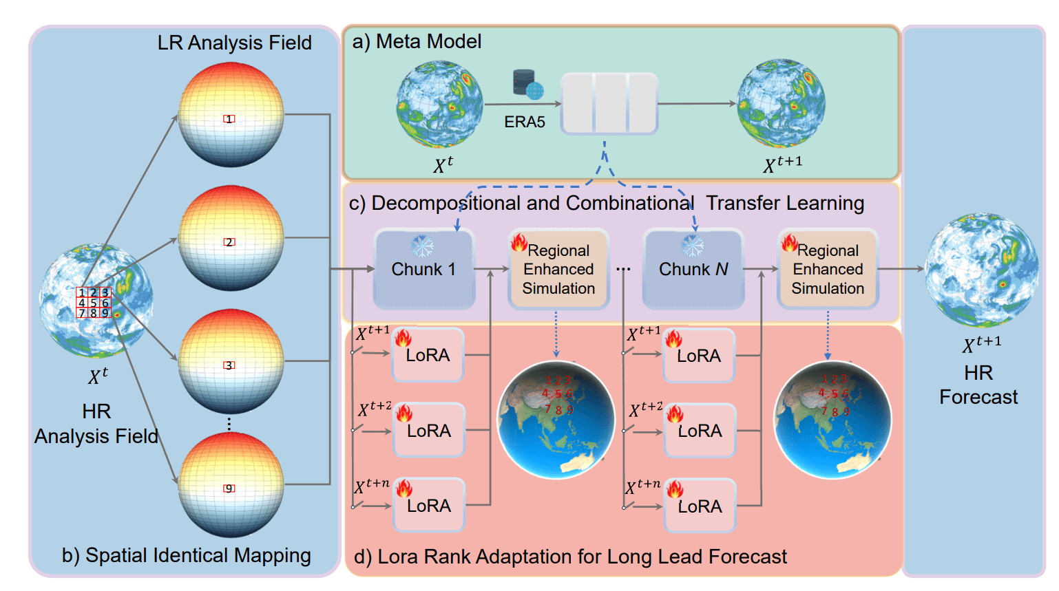
Figure 12: Low-Rank Adaptation is used to finetune for specific lead times (in red), while the original model remains the same. Image from Han et al. (2024).
Using diffusion models to sharpen forecasts
The focus of the approaches described previously was mostly reducing error accumulation for longer lead times. However, we also discussed that AI-based weather models are less expressive than NWP models when it comes to extreme weather conditions, which usually requires that small-scale phenomena are predicted precisely. The creators of the FuXi weather model recognize that diffusion models are used successfully in image generation (think the text-to-image tools available widely today) “due to their remarkable capability for generating highly detailed images” (Zhong et al., 2023). In other words, why not try and use them for sharpening weather forecasts?
In doing so, Zhong et al. (2023) use the outputs of FuXi as conditioning for a diffusion model trained to convert noise into surface-level weather variables. Now named FuXi-Extreme, significant performance improvements on metrics like CSI and SEDI are observed compared to the original FuXi model. In the figure below, especially around extreme weather events (such as cyclones present in Asia), predictions are clearly sharper.

Figure 13: applying a diffusion model trained on weather forecasts conditioned by outputs of the FuXi model (above) leading to sharper forecasts (below). Images from Zhong et al. (2023).
What’s next: AI-based ensemble weather modelling
This article demonstrates that limitations of AI-based weather modelling are not an end – but rather the start of often creative pursuits in finding solutions. In the next few articles, we will continue reviewing these developments. We start with AI-based ensemble modelling, where AI-based weather models are used to generate many forecasts at once, each with slight differences, allowing the uncertainty of weather predictions to be estimated. This is followed with AI-based limited-area modelling, as attempts are made to nest higher-resolution grids into AI-based weather models in different ways. Finally, the series is closed with a recap.
AI-based ensemble weather modelling
The weather is inherently uncertain. The speed with which AI-based weather forecasts can be generated enables scenario forecasting with significantly more scenarios to further reduce uncertainty. This is especially valuable in high-risk weather situations, such as when thunderstorms or windstorm systems threaten your operations.
AI-based limited-area modelling
Today’s AI-based weather models are global. Can we also extend AI-based weather forecasting to regional models with higher resolution? The answer is yes, as the first attempts to do this have emerged in research communities. In this article, we take a closer look at limited-area modelling with AI in this article.
A recap and future directions
With this article, the series on AI and weather forecasting comes to an end. We recap everything we have seen so far and use our broad understanding to draw future directions where developments can be expected.
Curious how AI-powered forecasts can support your operations? Let’s talk.

References
Bi, K., Xie, L., Zhang, H., Chen, X., Gu, X., & Tian, Q. (2022). Pangu-weather: A 3d high-resolution model for fast and accurate global weather forecast. arXiv preprint arXiv:2211.02556.
Chen, K., Han, T., Gong, J., Bai, L., Ling, F., Luo, J. J., ... & Ouyang, W. (2023a). Fengwu: Pushing the skillful global medium-range weather forecast beyond 10 days lead. arXiv preprint arXiv:2304.02948.
Chen, L., Zhong, X., Zhang, F., Cheng, Y., Xu, Y., Qi, Y., & Li, H. (2023b). FuXi: A cascade machine learning forecasting system for 15-day global weather forecast. npj Climate and Atmospheric Science, 6(1), 190.
Han, T., Guo, S., Ling, F., Chen, K., Gong, J., Luo, J., ... & Bai, L. (2024). Fengwu-ghr: Learning the kilometer-scale medium-range global weather forecasting. arXiv preprint arXiv:2402.00059.
Lam, R., Sanchez-Gonzalez, A., Willson, M., Wirnsberger, P., Fortunato, M., Alet, F., ... & Battaglia, P. (2022). GraphCast: Learning skillful medium-range global weather forecasting. arXiv preprint arXiv:2212.12794.
Versloot, C. (2021, July 19). How to use PyTorch loss functions. MachineCurve.com | Machine Learning Tutorials, Machine Learning Explained. https://machinecurve.com/index.php/2021/07/19/how-to-use-pytorch-loss-functions
Versloot, C. (2023, November 19). A gentle introduction to Lora for fine-tuning large language models. MachineCurve.com | Machine Learning Tutorials, Machine Learning Explained. https://machinecurve.com/index.php/2023/11/19/a-gentle-introduction-to-lora-for-fine-tuning-large-language-models
Versloot, C. (2024, June 27). AI & weather forecasting: Evaluate AI weather models with WeatherBench. Infoplaza - Guiding you to the decision point. https://www.infoplaza.com/en/blog/ai-weather-forecasting-evaluate-ai-weather-models-with-weatherbench
WeatherBench. (2024). Spectra. Spectra.
https://sites.research.google/weatherbench/spectra/
Zhong, X., Chen, L., Liu, J., Lin, C., Qi, Y., & Li, H. (2023). FuXi-Extreme: Improving extreme rainfall and wind forecasts with diffusion model. arXiv preprint arXiv:2310.19822.